
A
uburnUniversity
DepartmentofEconomics
WorkingPaperSeries
CollegeMajor,InternshipExperience,
andEmploymentOpportunities:
EstimatesfromaRésumé Audit
J
ohnM.Nunley,AdamPugh,Nicholas
Romero,andRichardAlanSeals,Jr.
A
U
WP2014‐03
Thispapercanbedownloadedwithoutchargefrom:
http://cla.auburn.edu/econwp/
http://econpapers.repec.org/paper/abnwpaper/

College Major, Internship Experience,
and Employment Opportunities:
Estimates from a R´esum´e Audit
John M. Nunley,
∗
Adam Pugh,
†
Nicholas Romero,
‡
and R. Alan Seals
§
March 30, 2014
¶
Abstract
We use experimental data from a r´esum´e-audit study to estimate the impact of par-
ticular college majors and internship experience on employment prospects. Our ex-
perimental design relies on the randomization of r´esum´e characteristics to identify the
causal effects of these attributes on job opportunities. Despite applying exclusively
to business-related job openings, we find no evidence that business degrees improve
employment prospects. Furthermore, we find no evidence linking particular degrees
to interview-request rates. By contrast, internship experience increases the interview-
request rate by about 14 percent. In addition, the “returns” to internship experience
are larger for non-business majors than for business majors.
JEL categories: J23, J24, J60
Key words: college major, internship, employment, field experiments, correspondence
studies, r´esum´e audit
∗
John M. Nunley, Department of Economics, University of Wisconsin—La Crosse, La Crosse, WI 54601,
†
Adam Pugh, Department of Economics, University of Wisconsin—La Crosse, La Crosse, WI 54601,
‡
Nicholas B. Romero, Department of Economics, University of Pennsylvania, Philadelphia, PA 19104,
graduate-program/current-students/nicholas-romero.
§
Richard Alan Seals Jr., Department of Economics, Auburn University, Auburn, AL 36849-5049, phone:
615-943-3911, email: alan.seals@auburn.edu, webpage: www.auburn.edu/ras0029.
¶
We thank the Office of Research and Sponsored Programs at the University of Wisconsin–La Crosse and
the Economics Department at Auburn University for generous funding. We thank Samuel Hammer, James
Hammond, Lisa Hughes, Amy Lee, Jacob Moore, and Yao Xia for excellent research assistance. We also
thank Erik Wilbrandt and Greg Gilbert for helpful comments.

1 Introduction
The reduction in initial employment opportunities for recent college graduates brought about
by the last recession has led many policymakers, researchers, and prospective students to
question the value of a college education. Popular internet newsboards regularly feature
articles that reference academic research on the projected labor-market demand for and life
satisfaction associated with certain undergraduate degrees. However, such information on
degree choice might be influenced by those who advertise on the same webpages that feature
the articles.
1
A large literature exists on the effects of college attendance, university quality, and degree
choice on labor-market outcomes (e.g., Oreopoulos and Petronijevic 2013; Altonji, Blom, and
Meghir 2012). However, the literature primarily focuses on life-cycle earnings and human-
capital acquisition rather than the effects of degree choice on labor demand (e.g., see Altonji,
Blom, and Meghir 2012). These studies also share a common limitation: the choice of
academic major could be driven by unobservables that make individuals more or less likely
to have success in the labor market.
Our study adds to the literature estimates of firms’ demand for job seekers with de-
grees in particular areas (e.g., business versus non-business). We implement an experimental
design that circumvents the identification issues in previous studies by randomly assigning
academic majors to fictitious job applicants. Our large-scale field experiment consists of sub-
mitting over 9000 randomly-generated r´esum´es to online job openings in banking, finance,
management, marketing, insurance and sales. The following academic majors are randomly
assigned to job applicants: accounting, biology, economics, english, finance, history, man-
agement, marketing, and psychology. We chose these academic majors because they are
common degree choices among college students. Because we apply exclusively for jobs in
1
For example, see the article and corresponding advertisments in the find-a-program tabs through the
following webpage: http://education.yahoo.net/articles/avoid_these_majors.htm.
1

business categories, we are particularly interested in whether the business degrees, i.e. ac-
counting, economics, finance, management and marketing, generate better job opportunities
than non-business degrees, i.e. biology, english, history, and psychology.
2
Another important feature of our experiment is the random assignment of internship
experience to a portion of the fictitious job seekers. The National Association of Colleges
and Employers’ (NACE) 2011 survey indicates that over 50 percent of graduating seniors
had worked as interns at some point while completing their degrees.
3
To our knowledge,
the economics literature has yet to focus on labor-market consequences associated with in-
ternship experience.
4
We believe that the absence of studies aimed at studying the impact
of internship experience on labor-market outcomes is due to either the lack of data or the
complications associated with identification. In the latter case, it is likely that high-ability
students are more likely to obtain internships and would also tend to have greater success
in the labor market. As such, a source of exogenous information or a structural model is
needed in order to identify the effect of internship experience on employment outcomes. In
our experiment, the random assignment of internship experience circumvents this problem,
allowing us to identify the causal effect of internship experience on job opportunities.
Despite applying exclusively to business-related job openings, we find no evidence that
employers prefer to interview job seekers with business degrees over applicants with non-
business degrees. In addition, there is no advantage, in terms of job opportunities, associ-
ated with a particular degree; that is, students with particular business degrees (e.g., finance,
marketing) fare no better than students with particular non-business degrees (e.g., english,
psychology). However, we find strong evidence that internship experience improves em-
2
It is not clear how to classify economics degrees, as it is a social science and many economics departments
are housed outside of business schools. We check the robustness of our estimates by including economics in
the non-business degree category, but the estimates are not sensitive to this reclassification.
3
For more details, visit the following webpage: http://www.schools.com/news/
survey-majority-of-internships-done-by-college-class-of-2011-were-paid.html.
4
Knouse, Tanner, and Harris (1999) use survey data to estimate the effect of internships on employment
outcomes. They find that internships increase employment opportunities for business majors; however, they
also find that those who receive internship experience had significantly higher grade point averages, which
suggests there may be estimation problems associated with self selection.
2

ployment prospects in economically and statistically significant ways. Applicants who were
assigned a three-month internship (Summer 2009) before they graduated with their Bache-
lor’s degrees (May 2010) receive about 14 percent more interview requests than those who
were not assigned internship experience. The “return” to internship experience is quite large
for both business and non-business majors, but it is economically larger for non-business-
degree holders than that for business-degree holders. To our knowledge, our study provides
the first set of estimates based on experimental data regarding the demand for job seekers
with particular college degrees and internship experience. More research is needed to bet-
ter understand the channels through which college degrees and internship experience affect
employment prospects.
2 Experimental Design
From January 2013 through the end of July 2013, we submitted approximately 9400 randomly-
generated, fictitious r´esum´es to online job openings in the following job categories: banking,
finance, insurance, management, marketing and sales. R´esum´es were submitted in the fol-
lowing cities: Atlanta, GA, Baltimore, MD, Boston, MA, Dallas, TX, Los Angeles, CA,
Minneapolis, MN and Portland, OR. The attributes listed on the r´esum´es were randomly
assigned to job seekers using the r´esum´e-randomizer developed by Lahey and Beasley (2009).
For each job advertisement, four r´esum´es were submitted. The following characteristics
were assigned to the fictitious job seekers: a name, a street address, a university where they
completed their Bachelor’s degree,
5
an academic major, (un)employment status, whether
they report their grade point average (GPA), whether the applicant graduated with an
Honor’s distinction, the type of work experience the applicant obtained after completing
their degree, and whether the applicant obtained internship experience while completing
5
It is important to point out that the universities that we used for this r´esum´e attribute are likely
recognizable to prospective employers, but it is unlikely that the universities would be regarded as prestigious.
In our regressions, we find that the interview rates do not vary between the four universities assigned to
applicants.
3

their degree. In the next paragraph, we describe the r´esum´e characteristics that are the focus
of this study (i.e. college major and internship experience). The other r´esum´e characteristics
mentioned above are described in Appendix B.
6
The first r´esum´e characteristic that is the focus of this study is college major. Applicants
are randomly assigned one of the following majors: accounting, biology, economics, english,
finance, history, management, marketing and psychology. Each of these majors are assigned
with equal probability. The second r´esum´e characteristic that is the focus of this study is
internship experience. In our experiment, 25 percent of applicants are assigned an “in-field”
internship that took place for three months during the summer (2009) prior to graduating
with their Bachelor’s degrees (May 2010). In our context, “in field” means that the internship
matches the job category. For example, internship experience is working as a(n) “Equity
Capital Markets Intern” in the banking job category; “Financial Analyst” in the finance job
category; “Insurance Intern” in the insurance job category; “Project Management Intern” or
“Management Intern” in the management job category; “Marketing Business Analyst Intern”
in the marketing job category; and “Sales Intern” or “Sales Future Leader Intern” in the sales
job category. Internship experience and college majors are assigned independent of each
other.
While the majority of the experiment is generated via the randomization of r´esum´e char-
acteristics, there are some features of the experiment that we had control over. First, all of
the fictitious job seekers graduated in May 2010. Second, the fictitious job seekers have one
job after graduating from college. Third, we applied to job openings in business-related job
categories. Fourth, we only applied to jobs that (a) required the submission of a r´esum´e to
be considered for the opening and (b) did not require a certificate or special training.
7
6
Appendix B, which provides detailed information on the experiment, is organized as follows. Section B1
provides detailed information on each of the r´esum´es characteristics; Section B2 provides examples of the
r´esum´es that were submitted to the job advertisements; and Section B3 details the process through which
applications were submitted.
7
With regard to (a), some job openings require that applicants complete a detailed firm-specific applica-
tion. We did not submit r´esum´es to these job advertisements for two reasons. First, the detailed application
introduces unwanted variation into the experimental design that is difficult to hold constant across appli-
cants. Second, the completion of detailed applications takes considerable time, and our objective was to
4

We measure employment opportunities by examining whether an applicant receives a
request for an interview from a prospective employer, which follows other researchers who
use the correspondence-audit framework (Baert et al. 2013; Bertrand and Mullainathan
2004; Carlsson and Rooth 2007; Eriksson and Rooth 2014; Kroft, Lange and Notowidigdo
2013; Lahey 2008; Oreopoulos 2011). We consider contact from a prospective employer an
interview request when they call or email to (a) schedule an interview and (b) discuss the
job opening in more detail. While the majority of the calls/emails received from employers
are classified as interview requests, there are a few instances in which the proper way to code
the inquiry from employers was unclear.
8
However, our estimates are not sensitive to ways
in which these questionable calls/emails are treated.
Table 1 presents the interview rates for applicants with all types of degrees (column 1);
business degrees (column 2); and non-business degrees (column 3). Table 1 is divided into
three panels. Panel A presents the interview rates for applicants with and without internship
experience; Panel B presents the interview rates for applicants without internship experience;
and Panel C presents the interview rates for applicants with internship experience. From
Panel A, the overall interview rate for business and non-business majors is 16.6 percent; the
interview rate for business majors is 17.0 percent; and the interview rate for non-business
majors is 16.2 percent. As a result, there appears to be little difference in the interview
rates between business and non-business majors. Indeed, the interview differential between
business and non-business majors is not statistically different from zero. From Panel B, a
similar pattern is observed: the interview rates for business majors without internship ex-
perience are slightly higher than that of non-business majors without internship experience
(16.7 percent versus 15.3 percent). In this case, the differential in interview rates between
generate as many data points as possible at the lowest possible cost.
8
Seventeen calls/emails, in particular, were difficult to classify in the “interview” or “non-interview” cat-
egories. These unclear “callbacks” consisted of employers asking whether the applicants were interested in
other positions; requesting salary requirements; asking whether the applicants were interested in part- or
full-time work; and inquiring about location preferences. In addition, there were 108 “callbacks” in which all
four applicants that were submitted to an advertisement received an call/email from employers. These 108
cases could be due to an automated response, or such callbacks could be non-discriminatory. Our estimates
are not sensitive to the ways in which these 125 employer responses are coded.
5

business and non-business majors is larger, but it is not statistically significant. From Panel
C, the overall interview rate for business and non-business majors with internship experience
is 18.4 percent, and non-business majors with internship experience have an interview rate
of 19 percent compared with 17.9 percent for business majors with internship experience. In
this case, the interview rate for non-business majors with internship experience is economi-
cally larger than that for business-majors, but, again, the difference between the two is not
statistically different from zero.
3 Results
The results section is divided into three subsections. Section 3.1 examines the impact of
college major on job opportunities; Section 3.2 examines the impact of internship experience
on job opportunities; and Section 3.3 examines whether there are interaction effects between
college major and internship experience.
3.1 College Majors and Job Opportunities
In this subsection, we investigate the impact of college major on job opportunities. We begin
by estimating the following regression model:
9
interview
imcfj
= β
0
+ β
1
bus
i
+ θX
i
+ φ
m
+ φ
c
+ φ
f
+ φ
j
+ u
imcfj
.
(1)
The subscripts i, m, c, f, and j index applicants, month of application, the city where the
application was submitted, the job category/field in which the application was submitted
and the job for which the application was submitted, respectively. The variable interview is
a zero-one indicator that equals one when an applicant receives an interview request and zero
9
All regression models are estimated using linear probability models. However, we check the robustness
of the marginal effects by estimating logit/probit specifications, finding similar results. In addition, standard
errors are clustered at the job-advertisement level in all model specifications.
6

otherwise; bus is a zero-one indicator that equals one when an applicant is assigned a business
degree (i.e. accounting, economics, finance, management or marketing) and zero otherwise;
10
X is a vector of r´esum´e characteristics that are randomly assigned to applicants;
11
φ
m
, φ
c
, φ
f
and φ
j
represent dummy variables for the month the r´esum´e was submitted, the city where
the r´esum´e was submitted, the job category that describes the job opening (i.e. banking,
finance, insurance, management, marketing and sales), and the job advertisement, respec-
tively. The β
0
, β
1
and θ are parameters to be estimated. We are particularly interested in
the parameter β
1
, which gives the average difference in the interview rate between applicants
with business degrees and applicants with non-business degrees.
Table 2 shows the estimates for β
1
from equation 1. There are six columns of estimates
presented in Table 2, which vary based on the control variables that are included in the
regression models. The estimates in column 1 include no control variables; the estimates in
column 2 condition on X; the estimates in column 3 condition on X and φ
m
; the estimates
in column 4 condition on X, φ
m
and φ
c
; the estimates in column 5 condition on X, φ
m
, φ
c
and φ
f
; and the estimates in column 6 condition on X, φ
m
, φ
c
, φ
f
and φ
j
. The estimates
for β
1
are remarkably stable as control variables are successively added to the regression
models. We find no evidence of a statistically significant link between business degrees and
interview rates. Furthermore, the practical size of the estimated differential is small and
(likely) economically insignificant.
The estimates presented in Table 2 suggest that business degrees do not materially affect
employment prospects, despite applying exclusively for business-related jobs. However, it is
possible that particular business degrees yield better job opportunities than particular non-
business degrees. Our next specification examines this possibility. Formally, we estimate the
10
As a robustness check, we estimate equation 1 with economics included in the non-business degree, given
that many economics departments are housed outside of business schools. However, in the majority of cases,
economics departments service business schools by teaching courses in the business curriculum. It is also
possible (perhaps likely) that the prospective employers in our sample view economics as a business-related
degree. In any case, the estimates are not sensitive to this alternative coding of the bus variable.
11
Detailed information on the r´esum´e attributes is provided in Section 2 and Appendix Section B1.
7

following regression equation:
interview
imcfj
= β
0
+ β
1
bio
i
+ β
2
eng
i
+ β
3
hist
i
+ β
4
psych
i
+ γ
1
actg
i
+ γ
2
fin
i
+ γ
3
mgt
i
+ γ
4
mkt
i
+ θX
i
+ φ
m
+ φ
c
+ φ
f
+ φ
j
+ u
imcfj
.
(2)
The subscripts i, m, c, f and j and the variables interview, X, φ
m
, φ
c
, φ
f
, φ
j
and u are
defined above. The variable bio is a zero-one indicator that equals one when an applicant
is assigned a degree in biology and zero otherwise; eng is a zero-one indicator that equals
one when an applicant is assigned a degree in english and zero otherwise; hist is a zero-
one indicator that equals one when an applicant is assigned a degree in history and zero
otherwise; psych is a zero-one indicator that equals one when an applicant is assigned a
degree in psychology and zero otherwise; actg is a zero-one indicator that equals one when
an applicant is assigned a degree in accounting and zero otherwise; fin is a zero-one indicator
that equals one when an applicant is assigned a degree in finance and zero otherwise; mgt is a
zero-one indicator that equals one when an applicant is assigned a degree in management and
zero otherwise; and mkt is a zero-one indicator that equals one when an applicant is assigned
a degree in marketing and zero otherwise. The base category in equation 2 is econ, which
is a zero-one indicator that equals one when an applicant is assigned a degree in economics
and zero otherwise. Because we are interested in creating an exhaustive set of comparisons
between applicants with particular business degrees and applicants with particular non-
business degrees, we can use the parameter estimates from equation 2 to construct linear
combinations of parameters with standard errors computed using the delta method.
12
For
example, the average difference in the interview rate between applicants with history degrees
relative to applicants with management degrees is β
3
− γ
3
. As another example, the average
difference in the interview rate between applicants with psychology degrees and applicants
12
In particular, we obtain the estimates for the linear combinations using the lincom command in STATA.
8

with finance degrees is β
4
− γ
2
.
13
Table 3 presents the estimated interview differentials between each non-business degree
and each business degree.
14
Equation 2 and the linear combinations of parameters described
above and in Appendix Table A1 are used to produce the estimates in Table 3. Rather
than comment on each of the estimates, it is sufficient to note that none of the academic
majors give job seekers an advantage in terms of job opportunities; that is, none of the
estimated interview differentials between the particular non-business and business degrees
are statistically significant.
15
The size of the estimated interview differentials vary depending
on the comparison being made. For the most part, the estimated differentials are unlikely
to be economically significant, as the majority of the estimates are less than 1.5 percentage
points (in absolute value). But there are a few exceptions.
Given that we apply to jobs across six different categories, it is possible that the “match”
between degree and job category matters. Our strategy to investigate this possibility is
to create a new variable that captures this idea. In particular, we estimate the following
regression model:
interview
imcfj
= β
0
+ β
1
match
i
+ θX
i
+ φ
m
+ φ
c
+ φ
f
+ φ
j
+ u
imcfj
.
(3)
The subscripts i, m, c, f and j and the variables interview, X, φ
m
, φ
c
, φ
f
, φ
j
and u are
defined above. The variable match is a zero-one dummy variable that equals one when the
applicant’s degree matches the job category. We use four different codings of the variable
13
Table A1 presents the remainder of the parameters and linear combinations of parameters of interest.
The parameters and linear combinations of parameters presented in Table A1 correspond to the estimates
presented in Table 3. Equivalently, we could change the base category and re-estimate equation 2 so that an
exhaustive set of comparions could be made.
14
The comparisons between particular business degrees (e.g., marketing versus finance) are presented in
Appendix Table A2, while the comparisons between particular non-business degrees (e.g., history versus
psychology) are presented in Appendix Table A3. The estimates presented in Tables A2 and A3 indicate no
statistical differences in the interview rates between the particular degrees.
15
When comparing the interview rates between applicants with specific degrees, the sizes of those cells
are quite a bit smaller than those for the business versus non-business degree comparisons. However, given
that each degree was assigned with a
1
/9 probability, there are over 1000 observations for each degree. Thus,
it is unlikely that the lack of statistical significance of the estimated differentials in Table 3 is due to small
sample sizes.
9
match in an attempt to gauge the sensitivity of the estimates. The first measure codes match
equal to one when the applicant’s degree is finance or economics in the banking and finance
job categories; when the applicant’s degree is management in the management job category;
and when the applicant’s degree is marketing in the marketing and sales job categories.
The second measure codes match equal to one when the applicant’s degree is finance or
economics in the banking, finance and insurance job categories; when the applicant’s degree
is management in the management job category; and when the applicant’s degree is marketing
in the marketing and sales job categories. The third measure codes match equal to one when
the applicant’s degree is finance or economics in the banking and finance job categories;
when the applicant’s degree is management in the management job category; and when the
applicant’s degree is marketing in the marketing job category. The fourth measure codes
match equal to one when the applicant’s degree is finance or economics in the banking,
finance and insurance job categories; when the applicant’s degree is management in the
management job category; and when the applicant’s degree is marketing in the marketing
job category. The estimate for β
1
gives the average difference in the interview rate for
applicants whose degrees match the job category and applicants whose degrees do not match
the job category.
Table 4 presents the estimates from equation 3. Column (1) presents the estimates using
the first definition of the match variable; column (2) presents the estimates using the second
definition of the match variable; column (3) presents the estimates using the third definition
of the match variable; and column (4) presents the estimates using the fourth definition of the
match variable. While the size of the parameter estimates varies depending on the definition
of the match variable, none of the estimated interview differentials are statistically different
from zero. Similar to the estimates presented in Table 3, it is also difficult to argue that
the size of the estimated interview differentials based on the match variable are practically
important (i.e. less than 1.5 percentage points in absolute value).
10
3.2 Internship Experience and Job Opportunities
In this subsection, we analyze the impact of internship experience while completing one’s
degree on employment opportunities. Our baseline regression model is
interview
imcfj
= β
0
+ β
1
intern
i
+ θX
i
+ φ
m
+ φ
c
+ φ
f
+ φ
j
+ u
imcfj
.
(4)
The subscripts i, m, c, f and j and variables interview, X, φ
m
, φ
c
, φ
f
, φ
j
and u are defined
above. The variable intern is a zero-one indicator that equals one when an applicant has
internship experience and zero otherwise. The parameter β
1
gives the average difference
in the interview rate between applicants with internship experience and applicants without
internship experience.
There are six columns of results presented in Table 5, which vary based on the control
variables that are held constant. In particular, we begin with a simple bivariate model
that includes no controls (column 1), add r´esum´e-specific controls (X) (column 2), add the
month-of-application dummy variables (φ
m
) (column 3), add the city-of-application dummy
variables (φ
c
) (column 4), add the job-category dummy variables (φ
f
) (column 5), and add
the job-advertisement dummy variables (φ
j
) (column 6). We find strong evidence that intern-
ship experience improves employment opportunities: applicants with internship experience
have interview-request rates that are 14 percent (about 2.2 percentage points) higher than
that for applicants without internship experience. The estimated impact of internship ex-
perience on employment opportunities is quite stable as control variables are successively
added to the regression equation. The estimates in each of the six columns are statistically
significant at the 0.1 percent level.
In Table 6, we present estimates for the impact of internship experience on job opportu-
nities based on a variant of equation 4 which includes an interaction between intern and the
11

job category (φ
f
). Formally, we estimate the following regression equation:
interview
imcfj
= β
0
+ β
1
intern
i
+
P
f
λ
f
intern
i
× φ
f
+ θX
i
+ φ
m
+ φ
c
+ φ
f
+ φ
j
+ u
imcfj
.
(5)
The subscripts i, m, c, f and j and variables interview, intern, X, φ
m
, φ
c
, φ
f
, φ
j
and
u are defined above. The parameter β
1
gives the average difference in the interview rate
between applicants with and without internship experience in the job category not included
in φ
f
, while the linear combination of parameters β
1
+ λ
f
gives the average difference in the
interview rate between applicants with and without internship experience in the non-omitted
job categories.
16
The estimates for β
1
and the linear combinations β
1
+ λ
f
are presented in
Table 6. For the most part, we find evidence of better job opportunities for applicants with
internship experience across all job categories, except in the banking and marketing job
categories (columns 1 and 5).
17
Applicants with internship experience have a 2.9 percentage
point higher interview rate in the finance job category (column 2); a 2.8 percentage point
higher interview rate in the insurance job category (column 3); a 3.0 percentage point higher
interview rate in the management job category (column 4); and a 2.6 percentage point higher
interview rate in the sales job category (column 6). The estimates in columns (2), (3), and
(6) are statistically significant at the 10-, one-, and 10-percent levels, respectively. Although
estimated differential in column (4) is not statistically significant, internship experience has
the largest economic impact in this job category.
16
Our specification of equation 5 treats job openings in insurance as the omitted category. Thus, β
1
gives
the average difference in the interview rate between job seekers with and without internship experience in
the insurance job category. The linear combinations β
1
+ λ
f
capture the effects of internship experience in
the remaining five job categories (i.e. banking, finance, management, marketing and sales).
17
In the banking and marketing job categories, the lack of finding statistical evidence of interview differ-
entials between applicants with and without internship experience does not appear to reflect small sample
sizes, as the coefficient estimates do not appear to be important in an economic sense (0.001 in banking and
−0.002 in marketing).
12
3.3 College Majors, Internships and Job Opportunities
3.3.1 Business Degrees, Non-Business Degrees and Internships
In this subsection, we examine interactions between particular college degrees and internship
experience. We begin by estimating the following regression model:
interview
imcfj
= β
0
+ β
1
bus
i
+ β
2
intern
i
+ β
3
bus
i
× intern
i
+ θX
i
+ φ
m
+ φ
c
+ φ
f
+ φ
j
+ u
imcfj
.
(6)
The subscripts i, m, c, f and j and variables interview, bus, intern, X, φ
m
, φ
c
, φ
f
, φ
j
and
u are defined above. We are primarily interested in the parameter β
2
, the linear combina-
tion of parameters β
2
+ β
3
, and the difference-in-differences estimator β
3
. The parameter
β
2
gives the average difference in the interview rate between applicants with and without
internship experience who have non-business degrees; the parameter combination β
2
+ β
3
gives the average difference in the interview rate between applicants with and without in-
ternship experience who have business degrees; and the parameter β
3
gives the estimated gap
in employment opportunities between business majors with and without internship experi-
ence and non-business majors with and without internship experience. The aforementioned
estimates are presented in Table 7. Column (1) presents the estimates for β
2
; column (2)
presents the estimates for β
2
+β
3
; and column (3) presents the estimates for β
3
. Non-business
degree majors with internship experience have a 20 percent (about 3.2 percentage points)
higher interview rate than their non-business-degree counterparts without internship expe-
rience (column 1). Business majors with internship experience have an 8 percent (about 1.4
percentage points) higher interview rate than business majors without internships experience
(column 2). The estimated interview differential based on internship status is about 11-12
percent (about 1.8 percentage points) larger for non-business majors than that for business
majors, but it is not statistically different from zero (column 3).
13

3.3.2 Specific Degrees and Internships
Because there could be differences in the “return” to internships based on particular college
majors, we estimate a regression model that interacts the particular academic degrees with
internships experience. In order to investigate this, we estimate the following regression
equation:
interview
imcfj
= β
0
+ β
1
bio
i
+ β
2
eng
i
+ β
3
hist
i
+ β
4
psych
i
+ γ
1
actg
i
+ γ
2
fin
i
+ γ
3
mgt
i
+ γ
4
mkt
i
+ λ
1
bio
i
× intern
i
+ λ
2
eng
i
× intern
i
+ λ
5
hist
i
× intern
i
+ λ
4
psych
i
× intern
i
+ δ
1
actg
i
× intern
i
+ δ
2
fin
i
× intern
i
+ δ
3
mgt
i
× intern
i
+ δ
4
mkt
i
× intern
i
+ θX
i
+ φ
m
+ φ
c
+ φ
f
+ φ
j
+ u
imcfj
.
(7)
The subscripts i, m, c, f and j and variables interview, actg, bio, eng, f in, hist, mgt,
mkt, psych, intern, X, φ
m
, φ
c
, φ
f
, φ
j
and u are defined above.
18
As in equation 3, the
base category is job seekers with economics degrees (i.e. econ). Using equation 7, we are
interested in determining whether internship experience generates a larger “return” for each
of the non-business degrees (i.e. biology, english, history and psychology) relative to each of
the business degrees (accounting, economics, finance, management and marketing).
The estimates for the exhaustive set of business versus non-business degree comparisons
for applicants with internship experience are presented in Table 8.
19
It is important to
point out that the standard errors for each of the estimated interview differentials are quite
large. The inflated standard errors are due to the small numbers of observations in the cells
of interest. We have slightly over 1000 observations for each major. Because internship
experience was randomly assigned at a rate of 25 percent, we have roughly 250 applicants
18
Note that the variable intern is included in X instead of being explicitly written out in equation 7.
19
We summarize the parameters and linear combinations of parameters used to produce the estimates
presented in Table 8 in Appendix Table A4.
14

who have a given academic major with internship experience. Thus, when comparing two
majors with internship experience, we have roughly 500 observations with which to conduct
our empirical tests, which is about one-fourth the sample size when not factoring in whether
applicants have internship experience or not. Due to the relatively smaller sample sizes
within these cells, we emphasize that the estimates presented in Table 8 should be used as
a way to gauge economic significance, not statistical significance.
Table 8 shows the interview differentials between applicants with non-business and busi-
ness degrees who also have internship experience that is specific to the six job categories
(i.e. banking, finance, insurance, management, marketing and sales). The columns of Table
8 vary based on the business degree used as the comparison group; that is, we compare the
interview rates of biology, english, history and psychology majors with internship experi-
ence separately to those who have degrees in accounting, economics, finance, management
and marketing with internship experience. Positive (Negative) coefficients indicate that the
particular non-business degree generates a higher (lower) interview-request rate than the
particular business degree chosen as the comparison. Rather than comment on each esti-
mate, it is sufficient to note that it is generally the case that history and psychology, two
degrees in the social sciences, generate economically larger interview rates than each of the
business degrees. The only exception is finance, in which case the point estimate is positive
but not large in a practical sense. As a result, the larger“return”to non-business majors with
internship experience over that of business majors with internship experience (See Table 7)
appears to be driven by the larger benefits conferred on psychology and history majors (not
biology and english majors).
20
20
Appendix Tables A5 and A6 present the estimated interview differentials between particular-business-
degree holders (e.g., finance versus accounting) with internship experience and particular-non-business-degree
holders (e.g., english versus biology) with internship experience, respectively.
15

4 Conclusions
We conduct a resume-audit designed to study the impact of college majors and internship
experience on job opportunities, which is measured via a request for an interview from
prospective employers. Despite applying exclusively to business-related jobs, we find no
evidence linking business degrees in general or particular business degrees to better job op-
portunities. However, we find strong evidence that internship experience has a large, positive
effect on employment opportunities. Job seekers with internship experience, obtained while
completing one’s college degree, have interview rates approximately 14 percent higher than
those without internship experience. The positive effects of internship experience are greater
for those who obtain non-business degrees. These results suggest that the current literature
on degree choice (e.g., Altonji, Blom, and Meghir 2004) should also consider work experience
during college and other extra-curricular activities.
21
It is important to note that we apply
for and receive interview requests between three and four years after the applicants’ college
degrees were received and between four and five years since the applicants worked as interns
in Summer 2009.
Our data suggest that college majors, assuming they have an immediate effect on initial
placement for the industries that we targeted, no longer have an impact of interview-request
rates three to four years after graduation. This is not the case for internship experience.
We identify an economically important effect four to five years after the internship ended.
These are interesting findings, but more research is needed to better understand the chan-
nels through which particular college majors and internship experience affect employment
opportunities. The key question regarding the findings for internship experience is whether
that attribute serves as a signal of ability or expected productivity or if it actually improves
the productivity of workers. The internship could also serve as an indicator of a high-quality
match between a firm and a job seeker (e.g., the applicant has worked in a bank as an intern
21
Oreopoulos (2011), however, finds no evidence that extra-curricular activities have an impact on subse-
quent employment prospects.
16
and he/she has indicated a preference to continue working in the banking sector by applying
years after the internship). One key estimation problem to overcome for future research is
to control for the heterogeneity of internships, as in the literature on apprenticeships (e.g.,
Adda, Dustman, Meghir, and Robin. 2013; Fersterer, Pischke, Winter-Ebmer 2008). There
are likely important interaction effects between degree choice, internship experience, and
other extra-curricular activities that could be captured in future studies.
References
[1] Adda, Jerome, Christian Dustman, Costas Meghir, and Jean-Marc Robin. 2013.“Career
Progression, Economic Downturns, and Skills.”NBER Working Paper Series No. 18832.
[2] Altonji, Joseph G., Erica Blom, and Costas Meghir.2012. ”Heterogeneity in Human
Capital Investments: High School Curriculum, College Major, and Careers.” Annual
Review of Economics, 4(1): 185-223.
[3] Bertrand, Marianne and Sendhil Mullainathan. 2004. “Are Emily and Greg More Em-
ployable than Lakisha and Jamal? A Field Experiment on Labor Market Discrimina-
tion.” American Economic Review, 94(4): 991-1013.
[4] Carlsson, Magnus, and Dan-Olof Rooth. 2007.“Evidence of Ethnic Discrimination in the
Swedish Labor Market Using Experimental Data.” Labour Economics, 14(4): 716-729.
[5] Eriksson, Stefan and Dan-Olof Rooth. 2011.“Do Employers Use Unemployment as Sort-
ing Criterion When Hiring? Evidence from a Field Experiment.” American Economic
Review, 104(3): 1014-1039.
[6] Fersterer, Josef, J
¨
orn-Steffen Pischke, Rudolf Winter-Ebmer. 2008. “Returns to Ap-
prenticeship Training in Austria: Evidence from Failed Firms.” Scandinavian Journal
of Economics, 110(4): 733-753.
[7] Knouse, Stephen B., John R. Tanner, and Elizabeth W. Harris. 1999. “The Relation of
College Internships, College Performance, and Subsequent Job Opportunity.” Journal
of Employment Counseling, 36(1): 35–43.
[8] Kroft, Kory, Fabian Lange and Matthew J. Notowidigdo. 2013. “Duration Dependence
and Labor Market Conditions: Theory and Evidence from a Field Experiment.” Quar-
terly Journal of Economics, 128(3): 1123-1167.
[9] Lahey, Joanna. 2008. “Age, Women and Hiring: An Experimental Study.” Journal of
Human Resources, 43(1): 30-56.
17
[10] Lahey, Joanna and Ryan A. Beasley. 2009. “Computerizing Audit Studies.” Journal of
Economic Behavior and Organization, 70(3): 508-514.
[11] Oreopoulos, Phillip. 2011. “Why Do Skilled Immigrants Struggle in the Labor Market?
A Field Experiment with Thirteen Thousand R´esum´es.” American Economic Journal:
Economic Policy, 3(4), 148-71.
[12] Oreopoulos, Philip, Till von Wachter, and Andrew Heisz. 2012. “The Short and Long-
Term Effects of Graduating in a Recession.” American Economic Journal: Applied Eco-
nomics, 4(1): 1-29.
[13] Oreopoulos, Phillip and Uros Petronijevic. 2013. “Making College Worth It: A Review
of Research on the Returns to Higher Education.”NBER Working Paper Series No.
1 9053.
18

Table 1: Summary Statistics
Business and
Non-business Business Non-business
Degrees Degrees Degrees
(1) (2) (3)
Panel A: Overall
Interview Rate 16.6% 17.0% 16.2%
Observations 9396 5189 4207
Panel B: Without Internships
Interview Rate 16.1% 16.7% 15.3%
Observations 7061 3875 3186
Panel C: With Internships
Interview Rate 18.4% 17.9% 19.0%
Observations 2335 1314 1021
19

Table 2: Difference Between Business and Non-Business Degrees
(1) (2) (3) (4) (5) (6)
Business Degree
0.007 0.008 0.008 0.007 0.007 0.004
(0.008) (0.008) (0.008) (0.008) (0.008) (0.007)
Controls:
R´esum´e No Yes Yes Yes Yes Yes
Month No No Yes Yes Yes Yes
City No No No Yes Yes Yes
Category No No No No Yes Yes
Advertisement No No No No No Yes
R
2
0.001 0.006 0.008 0.019 0.045 0.724
Observations 9396 9396 9396 9396 9396 9396
Notes: Estimates are marginal effects from linear probability models. Standard errors clustered at
the job-advertisement level are in parentheses. Columns (1)-(6) differ based on the control variables
that are held constant. In column (1), we estimate a bivariate regression model that include no
control variables; column (2) adds controls for the ‘R´esum´e’ characteristics; column (3) adds controls
for the month in which the applications were submitted; column (4) adds controls for the city in
which the applications were submitted; column (5) adds controls for the job category that describes
the opening; and column (6) adds controls for the job advertisement.
20

Table 3: Differences Between Particular Business and Non-Business Degrees
Base Category
Accounting Economics Finance Management Marketing
(1) (2) (3) (4) (5)
Biology
-0.005 -0.018 -0.019 -0.010 -0.003
(0.013) (0.014) (0.013) (0.013) (0.014)
English
0.009 -0.004 -0.005 0.004 0.014
(0.013) (0.014) (0.013) (0.013) (0.014)
History
-0.008 -0.021 -0.023 -0.013 -0.000
(0.014) (0.014) (0.014) (0.014) (0.014)
Psychology
0.013 -0.004 -0.002 0.008 0.017
(0.013) (0.014) (0.014) (0.013) (0.014)
R
2
0.724 0.724 0.724 0.724 0.724
Observations 9396 9396 9396 9396 9396
Notes: Estimates are marginal effects from linear probability models. Standard errors clustered at the job-advertisement level are
in parentheses. Columns (1)-(5) differ based on the college major that is used as the comparison group. Each column of estimates
uses the full set of control variables (i.e. the r´esum´e characteristics and the dummy variables for the month, city, job category and
job advertisement.
21

Table 4: Impact of Degrees that Match the Job Category
(1) (2) (3) (4)
Match
0.005 0.013 0.003 0.014
(0.009) (0.009) (0.010) (0.009)
R
2
0.724 0.724 0.724 0.724
Observations 9396 9396 9396 9396
Notes: Estimates are marginal effects from linear probability models. Standard errors clustered at
the job-advertisement level are in parentheses. Columns (1)-(4) differ based on the definition of the
”match” variable, which is discussed in the text. Each column of estimates uses the full set of control
variables (i.e. the r´esum´e characteristics and the dummy variables for the month, city, job category
and job advertisement.
22

Table 5: Impact of Internship Experience
(1) (2) (3) (4) (5) (6)
Internship
0.023*** 0.023*** 0.023*** 0.023*** 0.023*** 0.022***
(0.006) (0.006) (0.006) (0.006) (0.006) (0.006)
Controls:
R´esum´e No Yes Yes Yes Yes Yes
Month No No Yes Yes Yes Yes
City No No No Yes Yes Yes
Category No No No No Yes Yes
Advertisement No No No No No Yes
R
2
0.001 0.006 0.008 0.019 0.045 0.724
Observations 9396 9396 9396 9396 9396 9396
Notes: Estimates are marginal effects from linear probability models. Standard errors clustered at the job-
advertisement level are in parentheses. *** indicates statistical significance at the 0.1 percent level. Columns
(1)-(6) differ based on the control variables that are held constant. In column (1), we estimate a bivariate
regression model that include no control variables; column (2) adds controls for the ‘R´esum´e’ characteristics;
column (3) adds controls for the month in which the applications were submitted; column (4) adds controls for
the city in which the applications were submitted; column (5) adds controls for the job category that describes
the opening; and column (6) adds controls for the job advertisement.
23

Table 6: Impact of Internship Experience by Job Category
Job Category
Banking Finance Insurance Management Marketing Sales
(1) (2) (3) (4) (5) (6)
Internship
0.001 0.029+ 0.028** 0.030 -0.002 0.026+
(0.016) (0.015) (0.010) (0.020) (0.023) (0.016)
R
2
0.724 0.724 0.724 0.724 0.724 0.724
Observations 9396 9396 9396 9396 9396 9396
Notes: Estimates are marginal effects from linear probability models. Standard errors clustered at the job-advertisement
level are in parentheses. + and ** indicate statistical signifance at the 10- and one-percent levels, respectively. Column
(1) presents the difference in the interview between applicants with internship experience and applicants without internship
experience without internships experience in the banking job category; column (2) presents the difference in the interview
between applicants with internship experience and applicants without internship experience without internships experience in
the finance job category; column (3) presents the difference in the interview between applicants with internship experience
and applicants without internship experience in the insurance job category; column (4) presents the difference in the interview
between applicants with internship experience and applicants without internship experience without internships experience in the
management job category; column (5) presents the difference in the interview between applicants with internship experience and
applicants without internship experience without internships experience in the marketing job category; and column (6) presents
the difference in the interview between applicants with internship experience and applicants without internship experience
without internships experience in the sales job category. Each column of estimates uses the full set of control variables (i.e. the
r´esum´e characteristics and the dummy variables for the month, city, job category and job advertisement.
24

Table 7: Impact of Internship Experience for Business and Non-Business Majors
Business
Degree
Relative to
Non-Business Business Non-Business
Degree Degree Degree
(1) (2) (3)
Internship
0.032** 0.014+ -0.018
(0.011) (0.009) (0.015)
R
2
0.725 0.725 0.725
Observations 9396 9396 9396
Notes: Estimates are marginal effects from linear probability models. Standard errors clustered at the job-advertisement
level are in parentheses. + and ** indicate statistical significance at the 10- and one-percent levels, respectively. Column (1)
gives the estimated difference in the interview rate between non-business majors with internship experience and non-business
majors without internship experience; column (2) gives the estimated difference in the interview rate between business majors
with internship experience and business majors without internship experience; and column (3) gives the difference in interview
rates between non-business majors with and without internship experience and business majors with and without internships
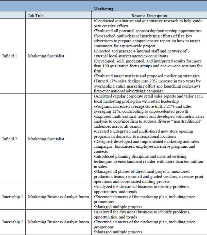
experience. The estimate in column (3) is, in effect, a difference-in-differences estimator. The estimates in columns (1)-(3)
are based on the same regression model, which uses the full set of control variables (i.e. the r´esum´e characteristics and the
dummy variables for the month, city, job category and job advertisement.
25

Table 8: Impact of Particular Business and Non-Business Degrees with Internships
Business Degree Used As Comparison Group
Accounting Economics Finance Management Marketing
(1) (2) (3) (4) (5)
Biology
0.006 -0.006 -0.022 -0.010 0.024
(0.029) (0.029) (0.029) (0.029) (0.030)
English
0.012 -0.000 -0.016 -0.004 0.029
(0.033) (0.033) (0.032) (0.033) (0.033)
History
0.038 0.026 0.009 0.021 0.056+
(0.032) (0.032) (0.032) (0.032) (0.033)
Psychology
0.032 0.032 0.003 0.016 0.050
(0.031) (0.031) (0.031) (0.031) (0.031)
R
2
0.725 0.725 0.725 0.725 0.725
Observations 9396 9396 9396 9396 9396
Notes: Estimates are marginal effects from linear probability models. Standard errors clustered at the job-advertisement level
are in parentheses. + indicates statistical significance at the 10-percent level. Each column of estimates uses a different business
degree as the base category (e.g., column 1 uses Accounting as the basis for comparison). The estimates in columns (1)-(5) are
based on the same regression model, which uses the full set of control variables (i.e. the r´esum´e characteristics and the dummy
variables for the month, city, job category and job advertisement.)
26

For Review Purposes Only
Appendix A: Supplementary Tables
Table A1: Parameters and Linear Combinations of Parameters for Table 3
Degree Used As Comparison Group
Accounting Economics Finance Management Marketing
(1) (2) (5) (7) (8)
Biology β
1
− γ
1
β
1
β
1
− γ
2
β
1
− γ
3
β
1
− γ
4
English β
2
− γ
1
β
2
β
2
− γ
2
β
2
− γ
3
β
2
− γ
4
History β
3
− γ
1
β
3
β
3
− γ
2
β
3
− γ
3
β
3
− γ
4
Psychology β
4
− γ
1
β
4
β
4
− γ
2
β
4
− γ
3
β
4
− γ
4
27

Table A2: Differences Between Particular Business Degrees
Degree Used As Comparison Group
Accounting Economics Finance Management
(1) (2) (3) (4)
Economics 0.014
– – –
(0.013)
Finance 0.014 0.001
– –
(0.013) (0.013)
Management 0.005 -0.008 -0.010
–
(0.013) (0.013) (0.013)
Marketing -0.005 -0.018 -0.019 -0.009
(0.013) (0.014) (0.014) (0.013)
R
2
0.724 0.724 0.724 0.724
Observations 9396 9396 9396 9396
28

Table A3: Differences Between Particular Non-Business Degrees
Degree Used As Comparison Group
Biology English History
(1) (2) (3)
English
0.014
– –
(0.013)
History
-0.003 -0.017
–
(0.014) (0.014)
Psychology
0.013 0.004 0.020
(0.013) (0.013) (0.014)
R
2
0.724 0.724 0.724
Observations 9396 9396 9396
29

Table A4: Parameters and Linear Combinations of Parameters for Table 7
Business Degree Used As Comparison Group
Accounting Economics Finance Management Marketing
(1) (2) (3) (4) (5)
Biology
β
1
+ λ
1
− (γ
1
+ δ
1
)
β
1
+ λ
1
β
1
+ λ
1
− (γ
2
+ δ
2
)
β
1
+ λ
1
− (γ
3
+ δ
3
)
β
1
+ λ
1
− (γ
4
+ δ
4
)
English
β
2
+ λ
2
− (γ
1
+ δ
1
)
β
2
+ λ
2
β
2
+ λ
2
− (γ
2
+ δ
2
)
β
2
+ λ
2
− (γ
3
+ δ
3
)
β
2
+ λ
2
− (γ
4
+ δ
4
)
History
β
3
+ λ
3
− (γ
1
+ δ
1
)
β
3
+ λ
3
β
3
+ λ
3
− (γ
2
+ δ
2
)
β
3
+ λ
3
− (γ
3
+ δ
3
)
β
3
+ λ
3
− (γ
4
+ δ
4
)
Psychology
β
4
+ λ
4
− (γ
1
+ δ
1
)
β
4
+ λ
4
β
4
+ λ
4
− (γ
2
+ δ
2
)
β
4
+ λ
4
− (γ
3
+ δ
3
)
β
4
+ λ
4
− (γ
4
+ δ
4
)
30

Table A5: Differences Between Particular Business Degrees
for Applicants with Internship Experience
Degree Used As Comparison Group
Accounting Economics Finance Management
(1) (2) (3) (4)
Economics
0.012
– – –
(0.026)
Finance
0.028 0.016
– –
(0.025) (0.026)
Management
0.016 0.004 -0.012
–
(0.025) (0.025) (0.024)
Marketing
-0.018 -0.030 -0.046+ -0.034
(0.027) (0.027) (0.027) (0.026)
R
2
0.724 0.724 0.724 0.724
Observations 9396 9396 9396 9396
31

Table A6: Differences Between Particular Non-Business Degrees
for Applicants with Internship Experience
Degree Used As Comparison Group
Biology English History
(1) (2) (3)
English
0.006
– –
(0.028)
History
0.032 0.026
–
(0.028) (0.031)
Psychology
0.026 0.020 0.016
(0.027) (0.030) (0.031)
R
2
0.724 0.724 0.724
Observations 9396 9396 9396
32

Appendix B: Data Appendix
B1 R´esum´e Characteristics
While details on the r´esum´e characteristics are provided in what follows, Table B1 summa-
rizes the variable names, definitions and provides the means of the variables. Some of the
variables are omitted from Table B1 (e.g., university that the applicant graduated from) per
our agreement with our respective institution review boards.
Applicant Names
Following the work of other correspondence studies (e.g., Bertrand and Mullainathan
2004; Carlsson and Rooth 2007; Nunley et al. 2011), we randomly assign names to applicants
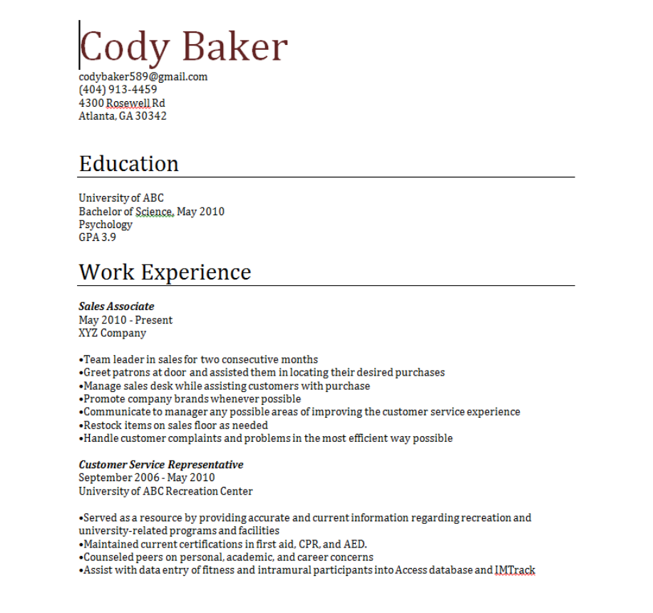
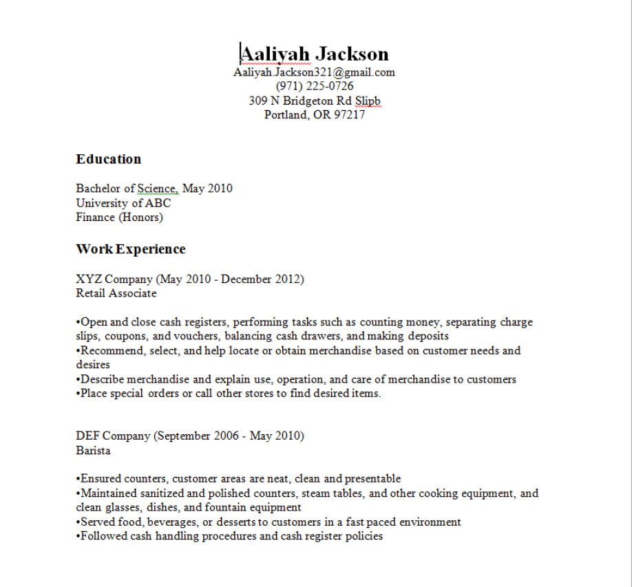
that are distinct to a particular racial group. For our purposes, we chose eight names:
Claire Kruger, Amy Rasumussen, Ebony Booker, Aaliyah Jackson, Cody Baker, Jake Kelly,
DeShawn Jefferson, and DeAndre Washington. Claire Kruger and Amy Rasmussen are
distinctively white female names; Ebony Booker and Aaliyah Jackson are distinctively black
female names; Cody Baker and Jake Kelly are distinctively white male names; and DeShawn
Jefferson and DeAndre Washington are distinctively black male names. The first names
and surnames were taken from various websites that list the most female/male and the
blackest/whitest names. The Census breaks down the most common surnames by race, and
we chose our surnames based on these rankings.
1
The whitest and blackest first names,
which are also broken down by gender come from the following website: http://abcnews.
go.com/2020/story?id=2470131&page=1. The whitest and blackest first names for males
and females are corroborated by numerous other websites and the baby name data from the
Social Security Administration.
The names listed above are randomly assigned with equal probability. Once a name has
been randomly assigned within a four-applicant group (i.e. the number of r´esum´es we submit
1
Here is the link to the most common surnames in the U.S.: http://www.census.gov/genealogy/www/
data/2000surnames/index.html.
33
per job advertisement), that name can no longer be assigned to the other applicants in the
four-applicant pool. That is, there can be no duplicate names within a four-applicant pool.
We created an email address and a phone number for each name, which were all created
through http://gmail.com. Each applicant name had an email address and phone number
that is specific to each city where we applied for jobs. As an example, DeAndre Washington
had seven different phone numbers and seven different email addresses. For each city, we
had the emails and phone calls to applicants within a particular city routed to an aggregated
Google account, which was used to code the interview requests.
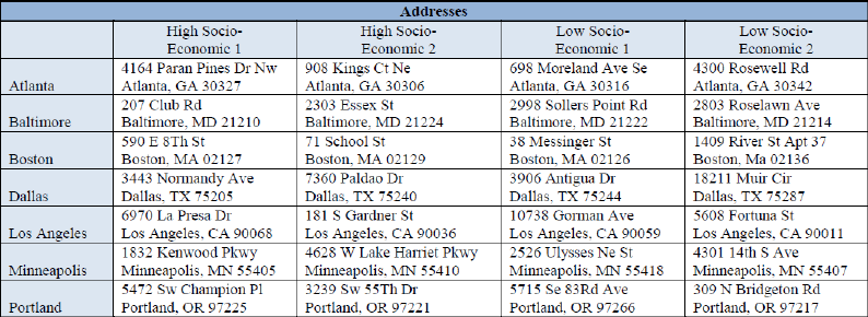
Street Address
Four street addresses were created for each city. The addresses are created by exam-
ining house prices in and around the city in which the applications are submitted. Two
of these addresses are in high-socioeconomic-status areas, while the other two are in low-
socioeconomic-status areas. High-socioeconomic-status addresses are in areas where house
prices on the street are in excess of $750,000, while those in low-socioeconomic-status ad-
dresses are in areas where house prices on the street are less than $120,000. We obtained
house price information from http://trulia.com. Each applicant is assigned one of the
four possible street addresses within each city. Applicants are assigned high- and low-
socioeconomic-status addresses with equal probability, i.e. 50 percent. The table below
shows the high- and low-socioeconomic street addresses used for each city.
34

Universities
The fictitious applicants were randomly assigned one of four possible universities. The
universities are likely recognizable by prospective employers, but they are unlikely to be
regarded as prestigious; thus, we can reasonably conclude that “name recognition” of the
school plays little role as a determinant of receiving a interview from a prospective employer.
In addition, each of the applicants is randomly assigned each of these four universities at
some point during the collection of the data. While the university one attends likely matters,
our data suggest that the universities that we randomly assigned to applicants do not give
an advantage to our fictitious applicants. That is, there is no difference in the interview rates
between the four possible universities.
Academic Major
The following majors were randomly assigned to our fictitious job applicants with equal
probability: accounting, biology, economics, english, finance, history, management, market-
ing, and psychology. We chose these majors because they are commonly selected majors by
college students. In fact, the Princeton Review
2
rates business-related majors as the most
selected by college students; psychology is ranked second; biology is ranked fourth; english
is ranked sixth; and economics is ranked seventh.
Grade Point Average and Honor’s Distinction
Twenty-five percent of our fictitious applicants are randomly assigned an r´esum´e attribute
that lists their GPA. When an applicant is randomly assigned this r´esum´e attribute, a GPA
of 3.9 is listed. Twenty-five percent of the fictitious applicants were randomly assigned
an Honor’s distinction for their academic major. Note that applicants were not randomly
assigned both of these attributes; that is, applicants receive one of the two or neither. Below
is an example of how the “Honor’s” (left) and “GPA” (right) traits were signaled on the
r´esum´es.
3
2
Visit the following webpage: http://www.princetonreview.com/college/top-ten-majors.aspx.
3
The university name was replaced with XYZ to conform to the terms of the agreement with our institu-
tional review boards.
35

(Un)Employment Status
Applicants were randomly assigned one of the following (un)employment statuses: em-
ployed at the date of application with no gap in work history, unemployed for three months
at the date of application, unemployed for six months at the date of application, unemployed
for 12 months at the date of application, unemployed for three months immediately follow-
ing their graduation date but currently employed, unemployed for six months immediately
following their graduation date but currently employed, and unemployed for 12 months im-
mediately following their graduation date but currently employed. Applicants receive no
gap in their work history at a 25 percent rate, while the different unemployment spells are
randomly assigned with equal probability (12.5 percent). The (un)employment statuses are
not mutually exclusive. It is possible for two workers in a four-applicant pool to be randomly
assigned, for example, a three-month current unemployment spell. The unemployment spells
were signaled on the r´esum´es via gaps in work history, either in the past or currently.
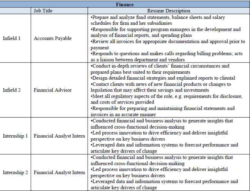
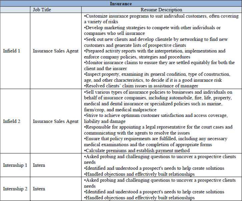
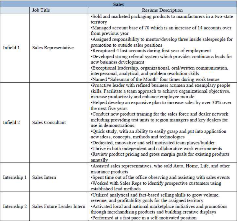
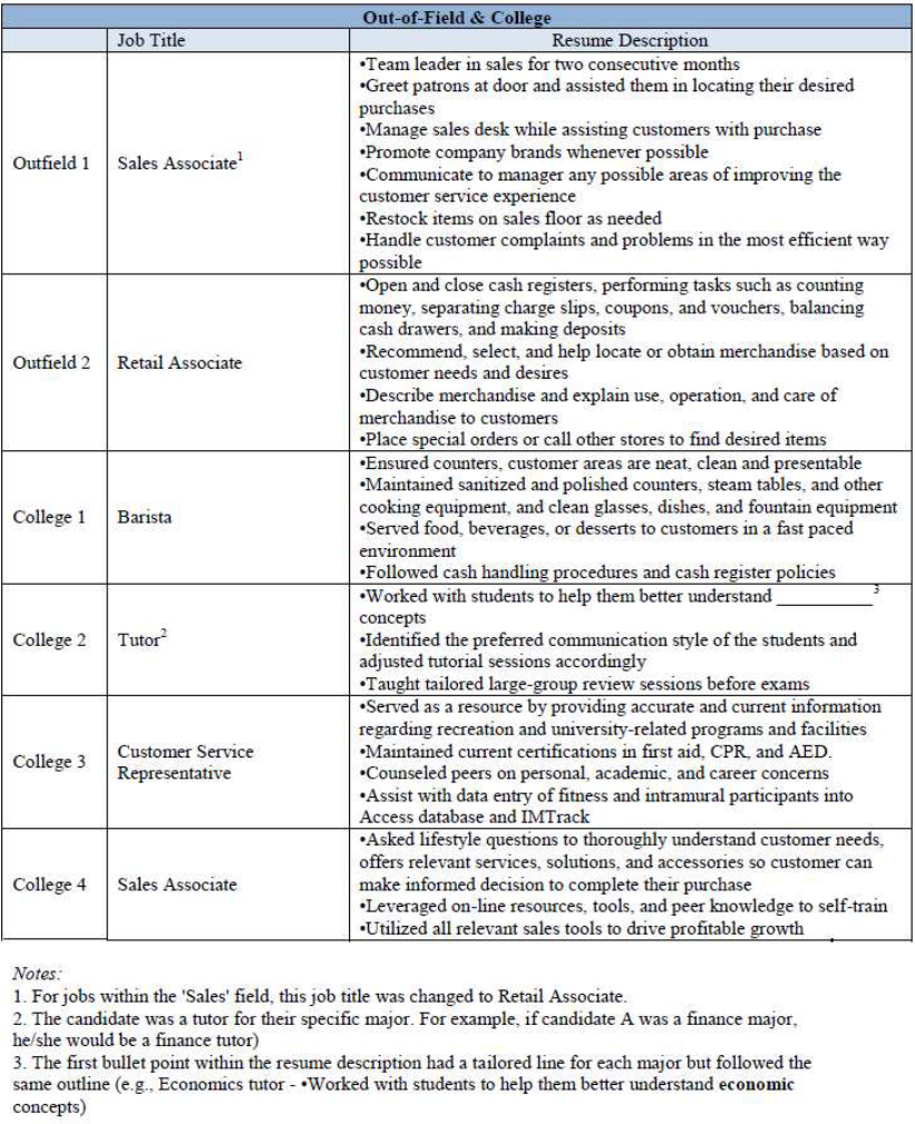
In-Field, Out-of-Field, Internship and College Work Experience
For each job category (i.e. banking, finance, management, marketing, insurance and
sales), applicants were randomly assigned “in-field” or “out-of-field” work experience. “In-
field” work experience is specific to the job category that the applicant is applying. “Out-
of-field” experience is either currently working or having previously worked as a sales person
in retail sales. Ultimately, out-of-field experience represents a form of “underemployment,”
as a college degree is not a requirement for these types of jobs. Fifty percent of applicants
are randomly assigned “in-field” experience, and the remaining 50 percent of applicants are
randomly assigned “out-of-field” experience. Twenty-five percent of the applicants were ran-
domly assigned internship experience during the summer 2009, which is the summer before
36
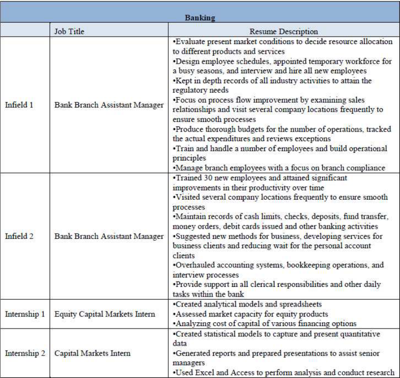
they completed their Bachelor’s degree. The internship experience is specific to the job cat-
egory. All of the applicants were assigned work experience while completing their college
degree, which consisted of working as a barista, tutor, customer service representative and
sales associate. The following series of tables provide detailed information on each type of
work experience by job category:
37
38
39
40
41
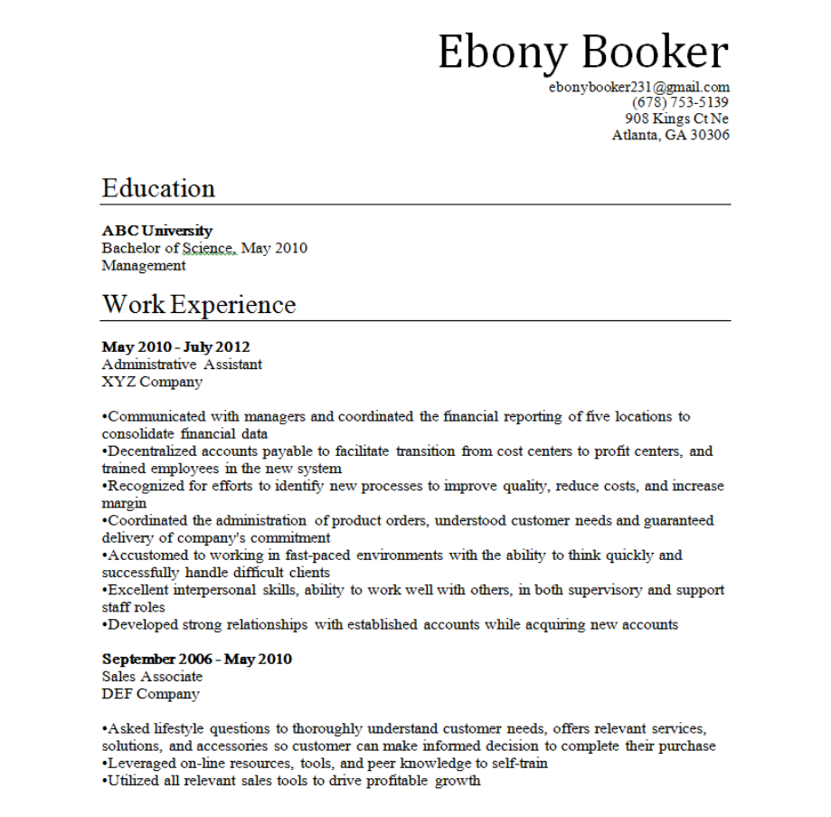
B2 Sample R´esum´es
In this section, we present a few r´esum´es that capture the essence of our r´esum´e-audit
study. The names of schools and companies where the applicants attended and worked have
been removed per our agreement with our respective institutional review boards.
42
43
44

45

46
B3 The Application Process
We applied to online postings for job openings in six categories: banking, finance, in-
surance, management, marketing and sales. To obtain an list of openings, we chose specific
search criteria through the online job posting websites to find the appropriate jobs within
each of the aforementioned job categories. We further constrained the search by applying
only to jobs that had been posted in the last seven days within 30 miles of the city center.
47
Job openings would be applied to if they had a “simple” application process. An application
process was deemed “simple” if it only required a r´esum´e to be submitted or if the informa-
tion to populate the mandatory fields could be obtained from the r´esum´e (e.g., a candidate’s
name or phone number). Jobs that required a detailed application were discarded for two
reasons. First and foremost, we wanted to avoid introducing variation in the application
process that could affect the reliability of our results. A detailed application specific to a
particular firm might include variation that is difficult to hold constant across applicants
and firms. Second, detailed applications take significant time, and our goal was to submit
a large number of r´esum´es to increase the power of our statistical tests. Job openings were
discarded from our sample if any of the following were specified as minimum qualifications:
five or more years of experience, an education level greater than a bachelor’s degree, unpaid
or internship positions, or specific certifications (e.g., CPA or CFA).
We used the r´esum´e-randomizer from Lahey and Beasely (2009) to generate four r´e-
sum´es to submit to each job advertisement. Templates were created for each job category
(i.e. banking, finance, insurance, management, marketing and sales) to incorporate in-field
experience. After the r´esum´es were generated, we then formatted the r´esum´es to look pre-
sentable to prospective employers (e.g., convert Courier to Times New Roman font; make
the applicant’s name appear in boldface font, etc.). We then uploaded the r´esum´es and filled
out required personal information, which included the applicant’s name, the applicant’s lo-
cation, the applicant’s desire to obtain an entry-level position, the applicant’s educational
attainment (i.e. Bachelor’s), and whether the applicant is authorized to work in the U.S.
All job advertisement identifiers and candidate information was recorded. Upon receiving
a interview request, we promptly notified the firm that the applicant was no longer seeking
employment to minimize the cost incurred by firms.
48

Table B1: R´esum´e Characteristics, Definitions, and Means
Variable Name Variable Definitions Mean
black =1 if applicant has a distinctively black name 0.497
female =1 if applicant has a distinctively female name 0.499
econ =1 if applicant has a Bachelor’s degree in Economics 0.115
finance =1 if applicant has a Bachelor’s degree in Finance 0.101
acctg =1 if applicant has a Bachelor’s degree in Accounting 0.112
mgt =1 if applicant has a Bachelor’s degree in Management 0.114
mkt =1 if applicant has a Bachelor’s degree in Marketing 0.111
eng =1 if applicant has a Bachelor’s degree in English 0.110
psych =1 if applicant has a Bachelor’s degree in Psychology 0.114
bio =1 if applicant has a Bachelor’s degree in Biology 0.116
hist =1 if applicant has a Bachelor’s degree in History 0.108
nogap =1 if applicant has a no gap in their work history 0.255
front3 =1 if applicant has a 3-month gap in their work history after finishing degree 0.125
front6 =1 if applicant has a 6-month gap in their work history after finishing degree 0.121
front12 =1 if applicant has a 12-month gap in their work history after finishing degree 0.125
back3 =1 if applicant has a current 3-month gap in their work history 0.124
back6 =1 if applicant has a current 6-month gap in their work history 0.123
back12 =1 if applicant has a current 12-month gap in their work history 0.127
intern =1 if applicant worked as an intern while completing their degree 0.248
infield =1 if applicant worked in the field for which they are applying for a job 0.500
highses =1 if applicant has an address in a high-socioeconomic-status area 0.499
honors =1 if applicant reports completing their degree with an Honor’s distinction 0.248
gpa =1 if applicant reports a grade point average (GPA) of 3.9 on their r´esum´e 0.249
exp Number of months that applicant has worked since completing their degree 30.02
49
